Introduction to Supervised Machine Learning

Roman Jurowetzki, 24. Sept. 2024

Introduction to Machine Learning

What is Machine Learning?

Some definitions that you will find out there.

• Algorithms that learn from data without explicit programming
• Improve performance with experience
• Automatically identify patterns and make decisions

Types of Machine Learning

1. Supervised Learning: Labeled data, predict outcomes
2. Unsupervised Learning: Unlabeled data, find patterns
3. Reinforcement Learning: Learn through interaction with environment
4. Self-Supervised Learning: Generate labels from the data itself

The Different Types of Learning

flowchart TD
    %% Nodes
    A("🧠 Supervised Learning")
    B("🔍 Unsupervised Learning")
    C("🤖 Self-Supervised Learning")
    D("🏷️ Labeled Data")
    E("📊 Unlabeled Data")
    F("⚙️ Model Training")
    G("✅ Evaluation")
    H("🧩 Pattern Discovery")
    I("🧬 Feature Learning")
    J("🎯 Predictions")
    K("📊 Clusters/Patterns")
    L("🧠 Learned Representations")

    %% Edge connections
    D ==> A ==> F
    E ==> B ==> H
    E ==> C ==> I
    F ==> G ==> |"Update Model"| F
    H ==> K
    I ==> L ==> |"Self-Supervision"| I
    F ==> J
    
    %% Styling
    style A fill:#e6f3ff,stroke:#0066cc,stroke-width:2px
    style B fill:#ffe6e6,stroke:#cc0000,stroke-width:2px
    style C fill:#e6ffe6,stroke:#006600,stroke-width:2px
    style D fill:#f0f0f0,stroke:#333333,stroke-width:2px
    style E fill:#f0f0f0,stroke:#333333,stroke-width:2px
    style F fill:#fff0e6,stroke:#ff6600,stroke-width:2px
    style G fill:#fff0e6,stroke:#ff6600,stroke-width:2px
    style H fill:#fff0e6,stroke:#ff6600,stroke-width:2px
    style I fill:#fff0e6,stroke:#ff6600,stroke-width:2px
    style J fill:#fff0e6,stroke:#0066cc,stroke-width:2px,stroke-dasharray:5 5
    style K fill:#fff0e6,stroke:#0066cc,stroke-width:2px,stroke-dasharray:5 5
    style L fill:#fff0e6,stroke:#0066cc,stroke-width:2px,stroke-dasharray:5 5

Supervised Machine Learning

Key Concepts

1. 🏋️‍♂️ Training data
2. 🏷️ Features and labels
3. 🧠 Model selection
4. 📉 Loss functions and optimization
5. 📊 Evaluation metrics
6. 🌐 Generalization

Add a brief explanation for each concept.

Mathematical Representation I

For a supervised learning problem:

• Input features: \(X = (x_1, x_2, ..., x_n)\)
  • A vector of n features for each data point
  • Example: For a house price prediction, \(x_1\) could be square meters, \(x_2\) number of rooms, etc.
• Target variable: \(y\)
  • The value we’re trying to predict
  • Example: The price of the house

Mathematical Representation II

• Model function: \(f(X)\)
  • The function that maps input features to predictions
  • Example: For linear regression, \(f(X) = w_0 + w_1x_1 + w_2x_2 + ... + w_nx_n\)
• Parameters: \(\theta\)
  • The values the model learns during training
  • Example: In linear regression, \(\theta\) would be the weights \((w_0, w_1, ..., w_n)\)

Mathematical Representation III

We aim to find \(f(X)\) such that:

\[y \approx f(X; \theta)\]

This means we want our model’s predictions \(f(X; \theta)\) to be as close as possible to the true values \(y\).

Explain that the goal of supervised learning is to find the function \(f\) and parameters \(\theta\) that make the best predictions. You might want to give a concrete example, like predicting house prices based on features like square footage, number of bedrooms, etc.

Loss Functions

Mean Squared Error (Regression)

\[MSE = \frac{1}{n}\sum_{i=1}^{n}(y_i - \hat{y_i})^2\]

Use case: Regression tasks. Measures how far the predicted values ( \(\hat{y_i}\) ) are from the actual values ( \(y_i\) ) by averaging the square of the differences. The larger the difference, the higher the penalty, as squaring the difference emphasizes bigger errors.

Cross-Entropy (Classification)

\[H(p,q) = -\sum_{x}p(x)\log q(x)\]

Use case: Classification tasks. Compares the true probability distribution ( \(p(x)\) ) (often 0 or 1 for classification) with the predicted probability ( \(q(x)\) ). If the predicted probability is far from the true label, it gives a higher penalty. Logarithms are used to give more emphasis to confident but wrong predictions.

• MSE is used when the output is continuous (e.g., predicting house prices).
• Cross-Entropy is used when the output is categorical (e.g., classifying images into cats or dogs).

Python Code for Loss Functions I

Mean Squared Error (MSE)

import numpy as np

# Actual and predicted values
y = np.array([3.5, 2.1, 4.0, 5.5, 6.1, 7.3, 3.9, 4.4, 5.0, 6.7])
y_hat = np.array([3.8, 2.0, 4.2, 5.0, 6.0, 7.5, 3.5, 4.2, 5.1, 6.8])

# Calculate MSE
n = len(y)
mse = (1/n) * np.sum((y - y_hat) ** 2)

\[MSE = \frac{1}{n}\sum_{i=1}^{n}(y_i - \hat{y_i})^2\]

Python Code for Loss Functions II

Cross-Entropy (Classification)

import numpy as np

# True labels (one-hot encoded) for 3 classes
p = np.array([
    [1, 0, 0],  # Class 1
    [0, 1, 0],  # Class 2
    [0, 0, 1],  # Class 3
    [1, 0, 0],  # Class 1
    [0, 1, 0],  # Class 2
])

# Predicted probabilities for each class (sum of each row should be 1)
q = np.array([
    [0.8, 0.1, 0.1],  # Predicted probabilities for Class 1, 2, 3
    [0.2, 0.7, 0.1],  # Predicted probabilities for Class 1, 2, 3
    [0.1, 0.2, 0.7],  # Predicted probabilities for Class 1, 2, 3
    [0.6, 0.3, 0.1],  # Predicted probabilities for Class 1, 2, 3
    [0.2, 0.6, 0.2],  # Predicted probabilities for Class 1, 2, 3
])

# Clip values to avoid log(0)
q = np.clip(q, 1e-12, 1 - 1e-12)

# Calculate cross-entropy for multiclass classification
cross_entropy = -np.sum(p * np.log(q))

\[H(p,q) = -\sum_{x}p(x)\log q(x)\]

Model Evaluation and Generalization

Train-Test Split

• Split data into training and test sets
• Train on training data
• Evaluate on test data
• Helps assess generalization

flowchart LR
    A[("🗄️ Dataset")]
    B["📊 Training Set\n80%"]
    C["🧪 Test Set\n20%"]
    D["🤖 Train the Model<br>Random Forest, XGBoost"]
    E["📈 Evaluate on Test Set<br>Accuracy, MSE, Precision"]
    F["🎯 Assess Generalization<br>Performance on unseen data"]
    
    A --> B
    A --> C
    B --> D
    D --> E
    C --> E
    E --> F
    
    classDef cool fill:#8EC5FC,stroke:#4A6FA5,stroke-width:2px,rx:10,ry:10;
    classDef warm fill:#FBC2EB,stroke:#A66E98,stroke-width:2px,rx:10,ry:10;
    classDef neutral fill:#E0EAFC,stroke:#8B9FBF,stroke-width:2px,rx:10,ry:10;
    
    class A,D cool;
    class B,C warm;
    class E,F neutral;

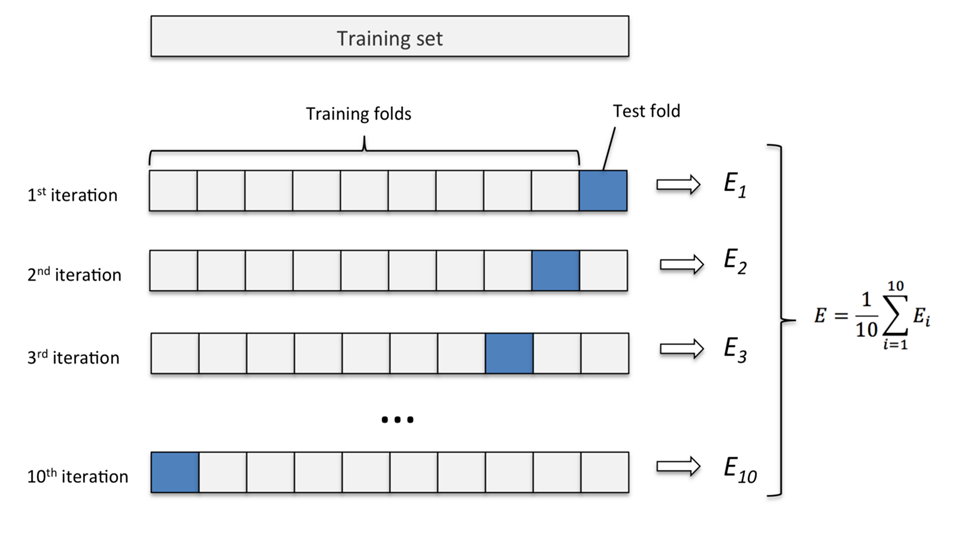
Cross-Validation

• K-fold cross-validation
• Helps in robust model evaluation
• Reduces overfitting

# Example code (not executed)
from sklearn.model_selection import cross_val_score
scores = cross_val_score(model, X, y, cv=5)
print(f"Cross-validation scores: {scores}")
print(f"Mean score: {scores.mean():.2f}")

Cross-Validation

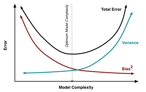
Bias-Variance Tradeoff

• Bias: Error from overly simplistic models (underfitting)

• Variance: Error from models too sensitive to training data (overfitting)

• Total Error = Bias² + Variance + Irreducible Error

  Goal: Find the optimal balance between bias and variance for the lowest possible total error.

This version adds more explanation to bias and variance, and highlights the purpose of the tradeoff.

Bias-Variance Tradeoff

Mathematical Representation of Bias-Variance

For a given point \(x\), the expected prediction error is:

\[E[(y - \hat{f}(x))^2] = \text{Var}(\hat{f}(x)) + [\text{Bias}(\hat{f}(x))]^2 + \text{Var}(\epsilon)\]

Where: - \(\text{Var}(\hat{f}(x))\) is the variance - \([\text{Bias}(\hat{f}(x))]^2\) is the squared bias - \(\text{Var}(\epsilon)\) is the irreducible error

Provide a simple interpretation of this equation.

Here’s how you could structure the slide:

Regularization: Preventing Overfitting

• Overfitting: When a model is too complex and memorizes training data, leading to poor performance on new data.
• Regularization: Technique to balance model complexity and performance, making the model generalize better.

Common Regularization Methods:

• Lasso (L1): Sets some coefficients to zero, ignoring less important features.
• Ridge (L2): Shrinks all coefficients, but keeps all features.
• Elastic Net: Combines both Lasso and Ridge regularization.

Elastic Net Formula

\[\lambda \sum_{p=1}^{P} [ (1 - \alpha) |\beta_p| + \alpha |\beta_p|^2]\]

• \(\lambda\): Controls regularization strength
• \(\alpha\): Balances L1 (Lasso) and L2 (Ridge)

Popular Model Classes

Linear Models

1. Linear Regression \[y = \beta_0 + \beta_1x_1 + \beta_2x_2 + ... + \beta_nx_n + \epsilon\]

2. Logistic Regression (for binary classification) \[P(y=1|X) = \frac{1}{1 + e^{-(\beta_0 + \beta_1x_1 + ... + \beta_nx_n)}}\]

3. Elastic Net

   • Combines L1 and L2 regularization

Add a brief real-world application for each model.

Tree-based Models

1. Decision Trees
   • Recursive binary splitting
   • Measures: Gini impurity, Information gain
2. Random Forests
   • Ensemble of decision trees
   • Bagging and feature randomness
3. Gradient Boosting Machines (e.g., XGBoost)
   • Sequential ensemble of weak learners
   • Optimizes a differentiable loss function

Decision Trees

graph TD
    A[Study Hours?] -->|Yes| B[Attendance?]
    A -->|No| C[Fail]
    B -->|High| D[Pass]
    B -->|Low| E[Fail]

    style A fill:#FFDDC1,stroke:#FFB3B3,stroke-width:2px;
    style B fill:#FFD9E8,stroke:#FFB3B3,stroke-width:2px;
    style C fill:#C7CEEA,stroke:#A3B3FF,stroke-width:2px;
    style D fill:#C7F9CC,stroke:#B2F2BB,stroke-width:2px;
    style E fill:#FFC9DE,stroke:#FFA1B5,stroke-width:2px;

Neural Networks

1. Multi-layer Perceptron (MLP)
   • Layers of interconnected neurons
   • Activation functions: ReLU, Sigmoid, Tanh
2. Recurrent Neural Networks (RNN)
   • Designed for sequential data
   • Long Short-Term Memory (LSTM) units
3. Transformers
   • Attention mechanisms for long-range dependencies
   • Used in NLP tasks (e.g., BERT, GPT) but also others
4. Graph Neural Networks (GNN)
   • For graph-structured data
   • Applications in social networks, biology

Practical Considerations

Feature Engineering

• Creating relevant features: Deriving new features to improve model performance.
• Handling missing data: Filling or removing incomplete data to ensure a robust model.
• Scaling and normalization: Ensuring features are on similar scales for algorithms that rely on distance (e.g., k-NN, SVM).

Example: One-Hot Encoding for Categorical Variables

Transforms categorical features into a numerical format that models can understand.

from sklearn.preprocessing import OneHotEncoder

# One-hot encoding example
encoder = OneHotEncoder(sparse=False)
X_encoded = encoder.fit_transform(X)

Model Selection and Tuning

• Cross-validation
• Hyperparameter optimization (e.g., Grid Search, Random Search)
• Ensemble methods

Example: Grid Search with cross-validation

# Example code (not executed)
from sklearn.model_selection import GridSearchCV
param_grid = {'C': [0.1, 1, 10], 'kernel': ['rbf', 'linear']}
grid_search = GridSearchCV(svm.SVC(), param_grid, cv=5)
grid_search.fit(X, y)

Conclusion

Key Takeaways

• ML learns patterns from data
• Supervised learning predicts outcomes
• Balance between bias and variance is crucial
• Model selection and evaluation are important
• Continuous learning and adaptation

Future Directions in ML

• AutoML
• Explainable AI (XAI)
• Few-shot and zero-shot learning
• Federated Learning
• AI Ethics and Fairness