In this session, you will:

1. Understand the characteristics of deep learning and be able to delineate it.
2. Get introduced to the history and general intuition of artificial neural networks
3. Grasp the benefits of deep learning
4. Understand the basic architecture of deep learning models

• In the past few years, artificial intelligence (AI) has been a subject of intense media hype.
• We’re promised a future of intelligent chatbots, self-driving cars, and virtual assistants
• A future sometimes painted in a grim light and other times as utopian, where human jobs will be scarce, and most economic activity will be handled by robots or AI agents.
• Just now: DALL-E, ChatGTP etc. amazes & frightens society, hinting towards great socio-technical-economic disruption top come.

• Notice: ML is just a particular subset of the realm of AI technologies and algorithms.
  
• Artificial Neural Networks in turn are just a subset of ML techniques.
• Deep Learning, again, is a subset, refering to a particular type of neural networks.

Long and rich history dating back to the 1940s. Three major waves of developments in deep learning:

1. Cybernetics: (1940s-1960s) has marked important developments in theories of biological learning and the training of simple models with a single neuron
2. Connectionism (1980s-1990s) has brought methodological advances that have allowed faster training of artificial neural networks with a few hidden layers
3. The ongoing wave that started around 2006 during which the appellative deep learning was coined.
4. 2015-2017: Modern Dl frameworks Tensorflow and PyTorch appear.
5. Now (2023) Generative models, diffusion models, and transformer have reached industry grade maturity.

• NNs in toy application around since the 1950s, but for a long time, the missing piece was an efficient way to train large neural networks.
• This changed in the mid-1980s, when multiple people independently rediscovered the Backpropagation algorithm - a way to train chains of parametric operations using gradient-descent optimization.
• First practical application in 1989 from Bell Labs: Yann LeCun combined convolutional neural networks and backpropagation to the problem of classifying handwritten digits. LeNet was used by the US Postal Service to automate the reading of ZIP codes on mail envelopes.
• Yet, lacking data, computing power, and the inability to extend beyond some simple applications led most researchers abandoning ANNs.
• Around 2010, only a number of people where still working on neural networks started to make important breakthroughs: the groups of Geoffrey Hinton at the University of Toronto, Yoshua Bengio at the University of Montreal, Yann LeCun at New York University, Dan Ciresan and IDSIA.
• In 2011, Dan Ciresan started winning image-classification competitions (ImageNet) with GPU-trained deep NNs. Then, Hinton’s group entered with convolutional neural networks, which dominated the competition ever since.
• Since, deep learning has also found applications in many other types of problems, such as NLP, and completely replaced SVMs and tree models in a wide range of applications.
• 2017: Combination of encoder/decoder architecture and self-attention mechanism in transformer models. Now the dominant architecture for all type of sequential/spatial problems.

• Faster computers (Moore’s law)
• More data (‘Data Is the New Oil in the Digital Economy’)
• Ecosystem & Software accessibility
• Methodological / algorithmic advances

• Artificial Neural Networks (ANNs) are the building blocks of deep learning systems.
• The term ‘neural network’ refers to neurobiology: central concepts in deep learning were developed in part by drawing inspiration from our understanding of the brain.
• However, this refers to an abstract and simplified inspiration, rather than the mimicing of human brain activity. They share some very basics, but are highly stilized.
• Its like saying a paper airplane is an artificial F20 fighter jet.
• Today, there is broad agreement in the scientific community that deep learning cannot be seen as an accurate model of how the brain actually works.
• Research trying to morre accurately mimic the brain architecture in DL models by now did not yield results.

Analogies with human brain:

• The units of calculation in an ANN are called neurons.
• The neurons are connected via synapses which are weighted.
• The network learns to accomplish a given task by adjusting these weights inputs.

• Somewhat like in the biological brain, NN model decision processes in the following steps:
  • Take input cells (neurons or units), and connect them to some output cell (in neuroscience, via a synapse)
  • The receiving cell’s input is equal to the submitting cell’s output, weighted by the strength of the connection
  • The cell transforms this input via a non-linear activation function to an output, which it in turn submits to other connected cells
• We refer to networks because the final architecture is obtained by composing together many different functions

• The goal of deep feedforward neural networks, also known as multilayer perceptrons (MLPs), is to approximate some function \(f^*\)
  • A feedforward network defines a mapping \(y = f(x; \theta)\) and learns the value of the parameter \(\theta\) that result in the best function approximation
  • Feedforward because information flows through the function being evaluated from \(x\), through the intermediate computation used to define \(f\), and finally to the output \(y\)

• The simplest architecture called perceptron. The model is associated with a directed acyclic graphs describing how functions are composed together.
• A perceptron can learn relatively simple functional forms.
• By adding additional layers, the exibility of the model can dramatically improve
• Additional layers can be understood as latent variables

Some methematical Intuition

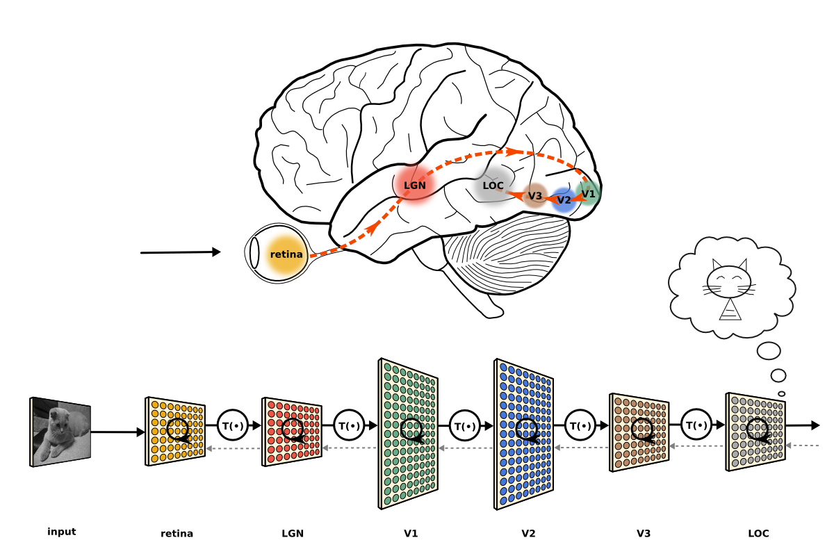
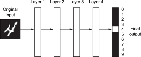
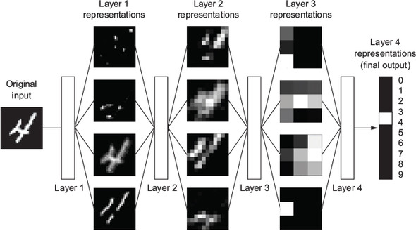
• Let us consider three functions \(f^{(1)}\), \(f^{(2)}\), and \(f^{(3)}\) connected in a chain, to form \(f(x) = f^{(3)}(f^{(2)}(f^{(1)}(x)))\)

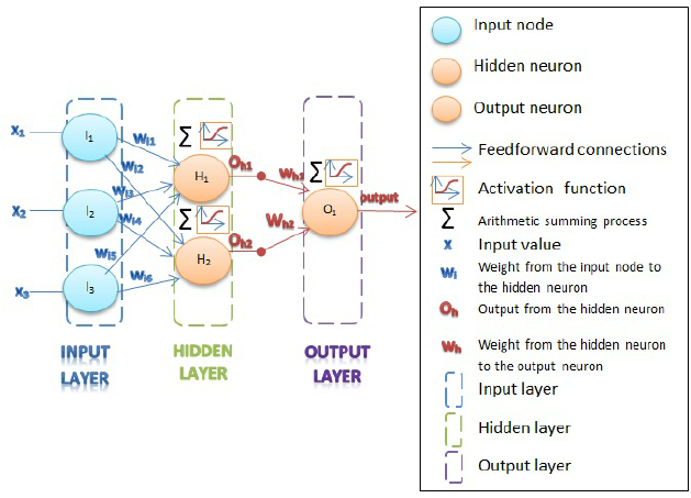
• \(f^{(1)}\) is called first layer (or input layer), \(f^{(2)}\) second layer (or first hidden layer), and so on… the overall length of the chain gives the depth of the model

• The final layer of the network is called the output layer \(f^*(x)\)

• During neural network training, we drive \(f(x)\) to match \(f^*(x)\)

• Because the training data does not show the desired output for each of the intermediate layers, these layers are called hidden layers

• The dimensionality of the hidden layers determines the width of the network

• Deep NNs overcome an obvious defect of linear models, that is their limited capacity to linear functions approximation; NN understand complex interactions between input variables.

Some common definitions:

• Deep learning can be viewed as a subset of machine learning methods aimed at processing large and complex datasets through networks of synthetic neurons. Here, subsequent layers learn increasingly abstract representations of the data that eventually become an input into predictions (Goodfellow, Bengio, and Courville, 2016)
  
• Deep learning allows computational models that are composed of multiple processing layers to learn representations of data with multiple levels of abstraction. (LeCun, Bengio, and Hinton, 2015)
• Deep learning, as it is primarily used, is essentially a statistical technique for classifying patterns, based on sample data, using neural networks with multiple layers […] Deep learning is a perfectly fine way of optimizing a complex system for representing a mapping between inputs and outputs, given a sufficiently large data set (Markus, 2018)

• So, whats the special thing about deep learning, and why is it deep anyhow?
• Conceptually, DL is a new take on learning representations from data that puts an emphasis on learning successive layers of increasingly meaningful representations, which is almost exclusively done via a neural network architecture.
• In contrast, most other ML approaches focus on learning only one or two layers of representations of the data \(\rightarrow\) shallow learning.

• What do the representations learned by a deep-learning algorithm look like?
• Let’s examine how a network several layers deep transforms an image of a digit in order to recognize what digit it is.

• The network transforms the digit image into representations that are increasingly different from the original image and increasingly informative about the final result.
• You can think of a deep network as a multistage information-distillation operation, where information goes through successive filters and comes out increasingly purified (that is, useful with regard to some task).
• So that’s what deep learning is, technically: a multistage way to learn data representations. It’s a simple idea-but, as it turns out, very simple mechanisms, sufficiently scaled, can end up looking like magic.

• Machine learning methods generally construct hypotheses directly from the data through inductive inference
  • If a large data set contains several instances of white swans and no instances of swans of other colours, a machine learning algorithm may infer that ‘all swans are white’
  • Inductive inferences consists of hypotheses which are always subject to falsification by additional data, i.e. there may still be an undiscovered island of black swans!
• Suppose the goal of a machine learning algorithm is to recognize a face in a picture, then the algorithm could use the presence of a nose as a feature.
  • Describing exactly what a nose is in terms of pixel composition can be difficult as there are countless different shapes, shadows can modify and obscure part of the nose, view angles, etc.
  • These attributes are known as factors of variations, i.e. constructs in the human mind that can be thought of as high-level abstractions that help us make sense of the rich variability of the observed data
  • A deep learning system learn from experience and understand the world in terms of a hierarchy of concepts, with each concept defined through its relation to simpler concepts

• Neural network architectures are the main drivers of latest hypes in AI and deep learning.
• They appear to have particular advantages in areas where the target function is subject to complex (eg. spatial, sequencial) interdependence, such as image and language data.
• Deep neural networks increase the available hypothesis space enourmeously.
• Deep neural networks typically need large amounts of data to be trained.
• Different architectural designs lead to performance advantage for particular types of problems.

• Bengio, Yoshua, Ian J. Goodfellow, and Aaron Courville. “Deep learning.” An MIT Press book. (2015). html (Deep Learning Bible)
• LeCun, Yann, Yoshua Bengio, and Geoffrey Hinton. “Deep learning.” Nature 521.7553 (2015): 436-444. pdf (Deep Learning Survey)
• Schmidhuber, Jürgen. “Deep learning in neural networks: An overview.” Neural networks 61 (2015): 85-117. pdf
• 3Blue1Brown: Best visual introduction to ANNs Youtube (Watch Chapter 1 for this session)