Updated February 02, 2023

This session

In this session, we will will:

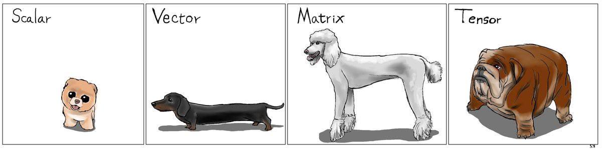
  1. Introduce tensors and tensor operations
  2. Be introduced to the basic building blocks of neural networks
  3. Get an insights how neural networks learn

Data representations for neural networks

Tensors

  • Most current DL frameworks use tensors as their basic data structure.
  • Tensors are fundamental to the field-so fundamental that Google’s TensorFlow was named after them. So what’s a tensor?
  • Tensors are a generalization of vectors and matrices to an arbitrary number of dimensions (note that in the context of tensors, a dimension is often called an axis). * A tensor is defined by three key attributes:
    1. Number of axes (rank): For instance, a 3D tensor has three axes, and a matrix has two axes.
    2. Shape: This is an integer vector that describes how many dimensions the tensor has along each axis.
    3. Data type: This is the type of the data contained in the tensor; for instance, a tensor’s type could be integer or double. On rare occasions, you may see a character tensor.

Tensors and dimensionality

  • Scalars (0D tensors): A tensor that contains only one number is called a scalar (or scalar tensor, or zero-dimensional tensor, or 0D tensor).
  • Vectors (1D tensors): A one-dimensional array of numbers is called a vector, or 1D tensor. A 1D tensor is said to have exactly one axis.
  • Matrices (2D tensors): A two-dimensional array of numbers is a matrix.
  • Arrays (3D and higher-dimensional tensors): If you pack such matrices in a new array, you obtain a 3D tensor. If you stack these arrays into another one, then you get a 4d tensor, and so forth…

Higher-dimensional tensors

  • Tensors of 3+d are used for many advanced applications, eg. timeseries, language and image processing.
  • For example, in the case before, we where working with 3d tensors, where the first two where a (greyscale pixel) matrix, and the third the different observations (samples) stacked on each others.
  • However, this greyscale raster matrix is somewhat a special case. Images typically have three dimensions: height, width, and color.
  • Therefore, a 2d image would therefore still represent a 3d tensor, and a bunch of them together a 4d tensor. For example, a batch of 128 RGB-color images could be stored in a 4d tensor of shape (128, 256, 256, 3)

  • 3d tensors are also often used for time series. Whenever time matters in your data (or the notion of sequence order), it makes sense to store it in a 3D tensor with an explicit time axis.
  • Each sample can be encoded as a sequence of vectors (a 2D tensor), and thus a batch of data will be encoded as a 3D tensor.
  • You might already see it coming…. colored videoes represent a time series of images, therefore would be a 5d tensor.
  • Videos can be seen as series of frames, where each frame can be stored in a 3D tensor 
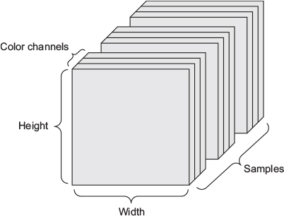
(height, width, color_depth), their sequence in a 4D tensor (frames, height, width, color_depth), and thus a batch of different videos in a 5D tensor of shape (samples, frames, height, width, color_depth).

Geometric interpretation of tensor operations

  • Because the contents of the tensors manipulated by tensor operations can be interpreted as coordinates of points in some geometric space, all tensor operations have a geometric interpretation. For instance, let’s consider addition.
  • We’ll start with the following vector: 
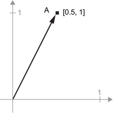
A = [0.5, 1.0]. It’s a point in a 2D space, but can also be under stood as a vector leading from the origin to this point.

  • Let’s consider a new point, 
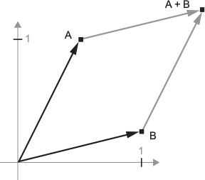
B = [1, 0.25], which we will add to the previous one. This is done geometrically by chaining together the vector arrows, with the resulting location being the vector representing the sum of the previous two vectors

  • In general, elementary geometric operations such as transformations, rotations, scaling, and so on can be expressed as tensor operations. For instance, a rotation of a 2D vector by an angle theta can be achieved via a dot product with a 2x2 matrix R = [u, v], where u and v are both vectors of the plane: u = [cos(theta), sin(theta)] and v = [-sin(theta), cos(theta)].
  • Some linear, vector and matrix algebra knowledge might light up again in your brain, right? Good! While for many out-of-the box “run-this-model” operations on tabular data, you might not need it, it will be necessary in case you need to tinker and customize a bit at your models to squeeze out a bit more accuracy.

Building blocks of networks

Overview

Layers: the building blocks of deep learning

  • A layer is a data-processing module that takes as input one or more tensors and that outputs one or more tensors.
  • Some layers are stateless, but more frequently layers have a state: the layer’s weights, one or several tensors learned with stochastic gradient descent, which together contain the network’s knowledge.
  • Different layers are appropriate for different tensor formats and different types of data processing. For instance, simple vector data, stored in 2D tensors of shape 
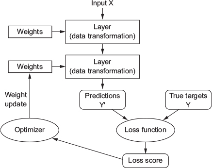
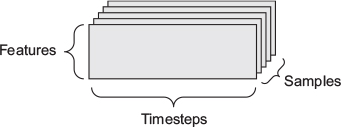
(samples, features), is often processed by densely connected layers, also called fully connected or dense layers (the layer_dense function in Keras).
  • Sequence data, stored in 3D tensors of shape (samples, timesteps, features), is typically processed by recurrent layers such as layer_lstm. Image data, stored in 4D tensors, is usually processed by 2D convolution layers (layer_conv_2d). All that will be introduced in later sessions.

  • You can think of layers as the LEGO bricks of deep learning, a metaphor that is made explicit by frameworks like 
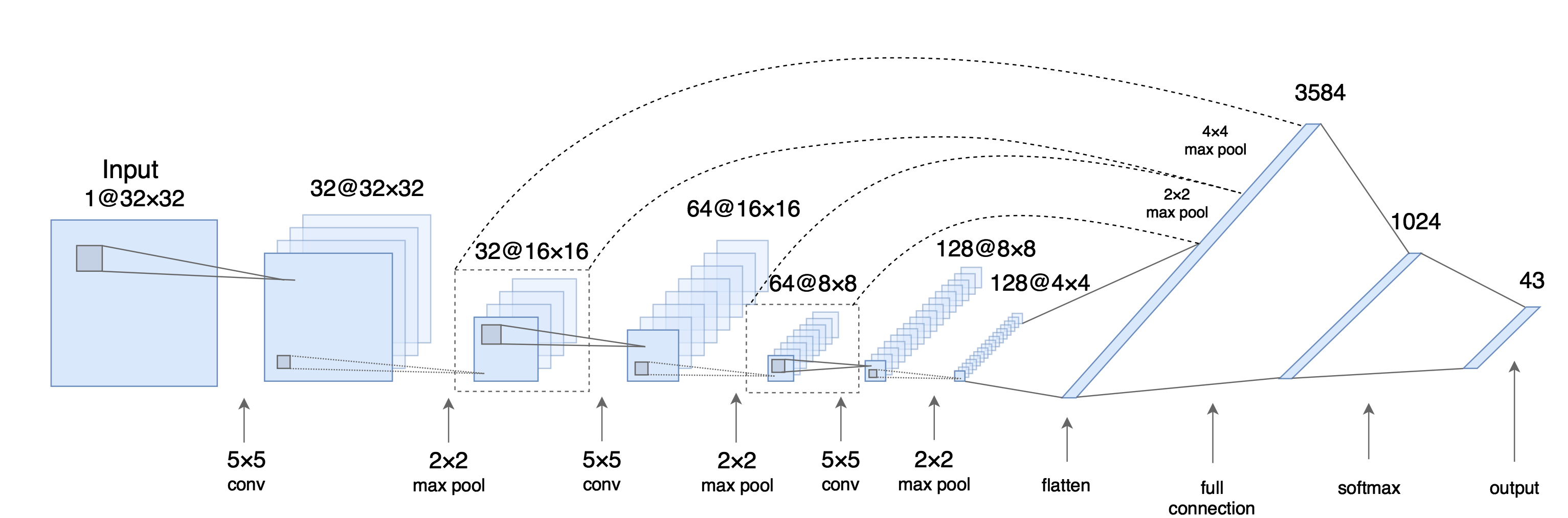
Keras. Pytorch has a more functional programming aspproach and abstraction, but still has the layeer-stacking narrative inbuilt.
  • Building deep-learning models in the different DL framework is done by clipping together compatible layers to form useful data-transformation pipelines.
  • The notion of layer compatibility here refers specifically to the fact that every layer will only accept input tensors of a certain shape and will return output tensors of a certain shape. Consider the example above.

Activation functions

  • Reminder: The weights which connect layers are as well tensors, which pass the output of the previous layer to the current one, where it gets transformed by the layer’s activation function.
  • Every cell gets 
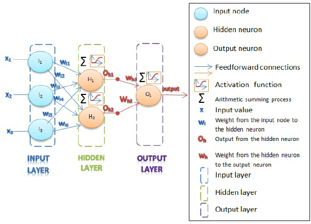
inputs from the connected other cells on lower layers which are activated, where the intensity of the input is scaled by the weight of the connection.

  • In feed-forward ANNs. Dense layers transforms its input data as follows: output = activation_function(dot(W, input) + b)
  • In this expression, W and b are tensors that are attributes of the layer.
  • They’re called the weights or trainable parameters of the layer (the kernel and bias attributes, respectively).
  • These weights contain the information learned by the network from exposure to training data.
  • The activation of every cell in the layer is therefore dependent on the multiplication of
    1. the corresponding input and weight tensor (dot(W, input))
    2. the bias (b), a constant which influences the tendency to activate.
  • Formally, Hidden units can be described as accepting a vector of inputs \(x\), compute an affine transformation \(z = W^T x + b\), and then applying an element-wise non-linear activation function \(g(z)\)
  • These activation functions are usually non-linear, since this increases the hypothesis space, allowing for more relationships than weighted-linear compositions
  • Historically, most prominent activation functions where:
    • Sigmoid function: \(g(z) = \sigma(z)\)
    • hyperbolic tangent: \(g(z) = \text{tanh}(z)\)
  • However, they turned out to saturate across most of their domain, making gradient-based learning very difficult

  • Nowadays, rectified linear units (ReLU) represents the most common FF-ANN activation function.
  • Here, the data is transformed linear, yet truncated at zero: \(h_i = g(z)_i = \text{max}(0,z_i)\)
  • ReLU is based on the principle that NNs are easier to optimize if their behaviour is closer to linear, yet still allows non-linearity.
  • Some generalizations of ReLU are based on using a nonzero slope \(\alpha_i\) when \(z_i < 0\) such that:
    • \(h_i = g(z,\alpha_i) = \text{max}(0,z_i) + \alpha_i \text{min}(0, z_i)\)
    • Absolute value rectification fixes \(\alpha_i = -1\) to obtain \(g(z) = |z|\)
    • Leaky ReLU fixes \(\alpha_i\) to a small value (e.g. 0.01)
    • Parametric ReLU (or PReLU) treats \(\alpha_i\) as a learnable parameter

Output (last layer activation)

  • The feedforward NN provides a set of hidden features defined by \(h = f(x); \theta)\). The output layer provides some additional transformation from the features to complete the task that the network must perform
  • For regression problems, we can use affine transformation with no non-linearity; these are just called linear units Given features \(h\), a layer of linear output units produces a vector \(\hat{y} = W^T h + b\). This produces the mean of a conditional distribution \(P(y|x)\)
  • For binary classification problems: The NN needs to predict \(P(y = 1 | x)\), so for this number to be a valid probability, it must lie in the interval \([0,1]\)
    • For this kind of problem, we use defined as: \(y = \sigma (w^T h + b)\), where \(\sigma\) is the logistic sigmoid function *This output unit has two components: first, it uses a linear layer to compute \(z = w^T h + b\); second, it uses the sigmoid activation function to convert \(z\) into a probability

  • To represent a probability distribution over a discrete variable with \(n\) possible values (multiclass) , we can use softmax output units (i.e. a generalization of the sigmoid function)
  • The goal is to produce a vector \(\hat{y}\), with \(\hat{y}_i = P(y = i | x)\) such that:
    • Each element of \(\hat{y}_i\) must lie in the interval [0,1]
    • The entire vector sums to 1
  • Again we have two steps: first, a linear layer predicts unnormalized log probabilities: \(z = W^T h + b\) where \(z_i = \text{log} \tilde{P}(y = i | x)\)
  • Second, the softmax function exponentiate and normalize \(z\) to obtain the desired \(\hat{y}\).
  • The softmax function is given by:

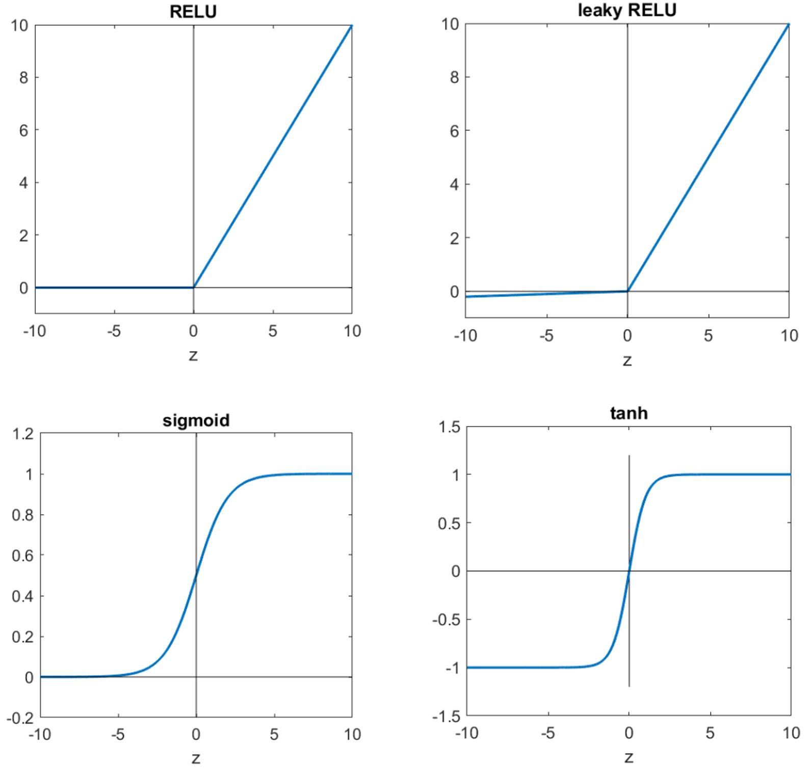
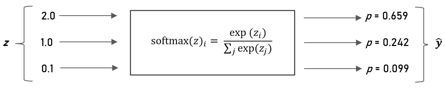
\(\text{softmax}(z)_i = \frac{\text{exp}(z_i)}{\sum_j \text{exp}(z_j)}\)

Loss functions

  • Another important element is the loss function, the quantity we want to minimize during the network training.
  • This is easy for linear (regression) problems, where one uses the well known mean- squared error (MSE), or mean absolute error (MAE)
  • For classification problems:
    • NNs define a distribution \(p(y|x;\theta)\) and we can use the principle of maximum likelihood
    • The cost function can be described as the **cross-entropy* between the training data and the model distribution
    • Formally, the cost function is given by:

\(J(\theta) = -\mathbb{E}_{x, y \sim \hat{p}_\text{data}} \text{log} \ p_\text{model} (y|x)\)

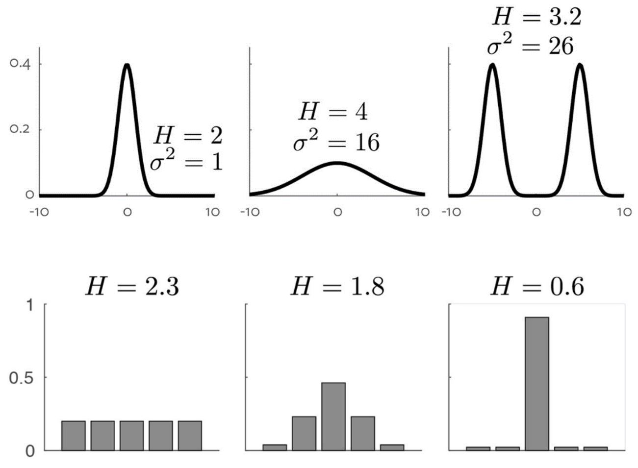
*Let’s go through some basic information theory

  • The basic intuition behind information theory is that learning that an unlikely even has occurred is more informative than learning that a likely event has occurred. That means:
    • Likely events should have low information content (or no information content whatsoever)
    • Less likely events should have higher information content
    • Independent events should have additive information
  • To satisfy the three properties, we can define the of an event \(\text{x} = x\) as: \(I(x) = -\text{log} P(x)\)
  • This definition is written in units of nats: one nat is defined as the amount of information gained by observing an event of probab. \(\frac{1}{e}\)
  • Self-information deals only with a single outcome; to quantify the amount of uncertainty in an entire probability distribution we can use the Shannon entropy
  • The Shannon entropy of a distribution is the expected amount of information in an event drawn from that distribution.
  • Distributions that are nearly deterministic have low entropy, whereas distributions that are closer to uniform have high entropy

\(H(\text{x}) = \mathbb{E}_{\text{x} \sim P} [I(x)] = - \mathbb{E}_{\text{x} \sim P} [\text{log} P(x)]\)

Summary

  • A little helper from my side ;). Works in most cases, at least for feedfoorward ANNs

Neural Network architecturas design

  • Architecture refers to the overall structure of the network: how many units it should have and how these units should be connected to each other
  • In chain-based architecture, the main considerations are choosing the depth of the network and the width of each layer
  • Generally, deeper networks use far fewer units per layer, generalize better to test sets, but they tend to be harder to optimize
  • The ideal architecture for a given task must be found via experimentation guided by monitoring its performance

  • Does learning complex input-output mappings require designing a specified model family for the kind of non-linearity we want to learn?
  • The universal approximation theorem states that a feedforward NN with a single hidden layer containing a finite number of units can approximate any continuous functions on compact subsets of \(\mathbb{R}^n\)
  • We are not guaranteed, however, that the training algorithm will be able to learn that function (optimization, overfitting)
  • To represent any function the hidden layer may be infeasibly large, hence using deeper models can reduce the number of units required to represent the desired function
  • Choosing deep models (instead of shallow networks) encodes a general belief that the function we want to learn can be viewed as a composition of several simpler functions
  • We believe the learning problem consists of discovering a set of underlying factors of variation that can in turn be described in terms of other, simpler factors of variation (i.e. edges, corners, contours, object parts, etc.)
  • Intermediate outputs are abstract concepts that the network uses to organize its internal processing
  • Empirically, greater depth seems to result in better generalization for a wide variety of tasks

  • Empirical results showing that deeper networks generalize better when used to transcribe multidigit numbers from photographs of addresses.

  • Empirical results showing that increasing the number of parameters in layers of convolutional neural networks without increasing their depth is not effective for increasing test set performance.

Learning in Neural Networks

The learning problem

  • So, now we know what the deep means, and how such a deep neutwork is structured. However, we still do not know so much about the learning.

  • Generally, learning appears in the network by adjusting the weights between the different cells.

  • But how does that happen?

  • Initially, these weight matrices are filled with small random values (a step called random initialization).

  • Of course, there is no reason to expect that relu(dot(W, input) + b), when W and b are random, will yield any useful representations.

  • What comes next is to gradually adjust these weights, based on some feedback signal (provided by the loss function).

  • This gradual adjustment, also called training, is basically the learning that ML is all about.
  • This happens within what’s called a training loop, which works as follows. Repeat these steps in a loop, as long as necessary:
    1. Draw a batch of training samples x and corresponding targets y.
    2. Run the network on x (a step called the forward pass) to obtain predictions y_pred.
    3. Compute the loss of the network on the batch, a measure of the mismatch between y_pred and y.
    4. Update all weights of the network in a way that slightly reduces the loss on this batch.
  • Step 1 sounds easy enough-just I/O code.
  • Steps 2 and 3 are merely the application of a handful of tensor operations, so you could implement these steps purely from what you learned in the previous section.
  • The difficult part is step 4: updating the network’s weights. Given an individual weight coefficient in the network, how can you compute whether the coefficient should be increased or decreased, and by how much?
  • The currently dominnat approach to do so is to take advantage of the fact that all operations used in the network are differentiable, and compute the gradient of the loss with regard to the network’s coefficients. You can then move the coefficients in the opposite direction from the gradient, thus decreasing the loss.
  • Lets take a step back…

Refresher What’s a derivative?

  • Consider a continuous, smooth function f(x) = y, mapping a real number x to a new real number y.
  • Because the function is continuous, a small change in x can only result in a small change in y.
  • Let’s say you increase x by a small factor epsilon_x: this results in a small epsilon_y change to y:

f(x + epsilon_x) = y + epsilon_y

  • In addition, because the function is smooth (its curve has no abrupt angles), when epsilon_x is small enough, around a certain point p, it’s possible to approximate f as a linear function of slope a, so that epsilon_y becomes a * epsilon_x:

f(x + epsilon_x) = y + a * epsilon_x

  • Obviously, this linear approximation is valid only when x is close enough to p. The slope a is called the derivative of f in p.

  • For every differentiable function 
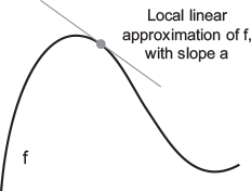
f(x), there exists a derivative function f'(x) that maps values of x to the slope of the local linear approximation of f in those points.
  • If you’re trying to update x by a factor epsilon_x in order to minimize f(x), and you know the derivative of f, then your job is done: the derivative completely describes how f(x) evolves as you change x.
  • If you want to reduce the value of f(x), you just need to move x a little in the opposite direction from the derivative.
  • It is helpful to track cregions where f'(x)==0, since they indicate the directional change of the curvature, and therefore local maxima or minima of f(x).
  • Btw: The curvature of f(x) is found in its second derivative, f''(x).

Derivative of a tensor operation: the gradient

  • A gradient is the derivative of a tensor operation. Consider an input vector x, a matrix W, a target y, and a loss function loss.
  • You can use W to compute a target candidate y_pred, and compute the loss, or mismatch, between the target candidate y_pred and the target y:
    • y_pred = dot(W, x)
    • loss_value = loss(y_pred, y)
  • If the data inputs x and y are frozen, then this can be interpreted as a function mapping values of W to loss values:
    • loss_value = f(W)

Stochastic gradient descent

  • Since 
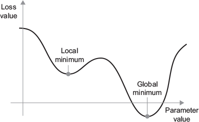
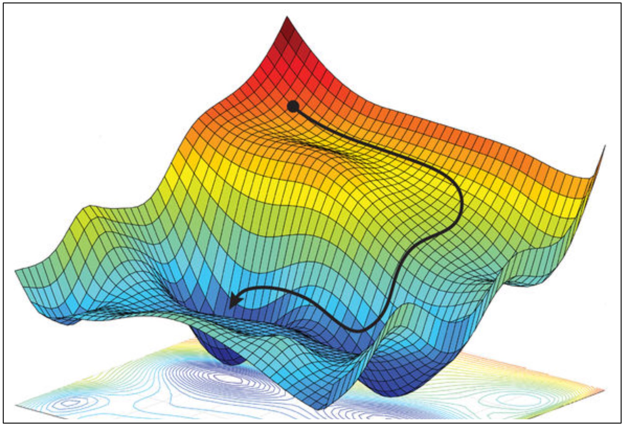
f'(x)==0indicates a local minimum, to find the global one we “only” need to identify all f'(x)==0 regions and check which has the lowest f(x).
  • Applied to a neural network, that means finding analytically the combination of weight values that yields the smallest possible loss.
  • To do so, we use the four-step algorithm outlined earlier: modify the parameters little by little based on the current loss value on a random batch of data.
  • Because you’re dealing with a differentiable function, you can compute its gradient, which gives you an efficient way to implement step 4.

If you update the weights in the opposite direction from the gradient, the loss will be a little less every time:

  1. Draw a batch of training samples x and corresponding targets y.
  2. Run the network on x to obtain predictions y_pred.
  3. Compute the loss of the network on the batch, a measure of the mismatch between y_pred and y.
  4. Compute the gradient of the loss with regard to the network’s parameters (a backward pass).
  5. Move the parameters a little in the opposite direction from the gradient-for example, W = W - (step * gradient) - thus reducing the loss on the batch a bit.

  • Easy enough! What we just described is stochastic gradient descent (mini-batch SGD).
  • The term stochastic refers to the fact that each batch of data is drawn at random (stochastic is a scientific synonym of random).
  • As you can see, intuitively it’s important to pick a reasonable value for the 
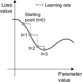
step, which we call the learning rate.
    • If it’s too small, the descent down the curve will take many iterations, and it could get stuck in a local minimum.
    • If step is too large, your updates may end up taking you to completely random locations on the curve.

  • There are many different ways to tinker with things like the learning rate and momentum (we call these ways of defining the learning function to find the global optimum optimizer), which influence how efficient the process leads (or not) to a global optimum.

The Backpropagation algorithm: Chaining derivatives

  • So, now we are almost there. We know now how to minimize the loss function within a layer.
  • However, the issue with deep learning is… well… that you have many layers.
  • How do we move on from here? Indeed, the rise of deep learning had to wait till the implementation of a efficient way to train multi-layered networks.
  • Luckily, we now have it, and its called backpropagation. And its actually pretty simple. While an enormous task in terms of number of calculations, the math behind it chould be acessible by highschool students.

  • Just imagine, we have a 4-layered network, connected by 4 weight tensors.

f(W1, W2, W3) = a(W1, b(W2, c(W3)))

  • Calculus tells us that such a chain of functions can be differentiated using the following identity, called the chain rule (ohh, dark memories, right?):

f(g(x)) = f'(g(x)) * g'(x)

  • Applying the chain rule to the computation of the gradient values of a neural network was one simple but brilliant ideas.
  • Now we can start with the last output layer, and propagate the loss via the chain rule step-by-step back over all weights in the leyer below, and then the one below etc., and adjust the weights accordingly.
  • Backpropagation starts with the final loss value and works backward from the top layers to the bottom layers, applying the chain rule to compute the contribution that each parameter had in the loss value.
  • Sounds like a hell to calculate by hand, right? Would be, but dont worry, you will not have to.

Summary: The parts of a deep learning model

Overview

  • As we understand by now training a neural network revolves around the following objects:
    1. The layers, which are combined into a network (or model)
    2. The input data and corresponding outcome targets
    3. The loss function, which defines the feedback signal used for learning
    4. The optimizer, which determines how learning proceeds
  • In interaction, it can be illustrated like this: The network, composed of layers that are chained together, maps the input data to outcomes of interest by doing predictions.
  • The loss function then compares these predictions to the targets, producing a loss value: a measure of how well the network’s predictions match what was expected.
  • The optimizer uses this loss value to update the network’s weights.

Appendix: Gradient Descent formulaic

Backpropagation formulaic

  • Weight matrices are filled with small random values (a step called random initialization)
  • The training loop consists of a gradual adjustment of the weights:
    • Draw a batch of training examples \(x\) and corresponding targets \(y\)
    • Run the network on \(x\) (a step called the forward pass) to obtain predictions \(\hat{y}\)
    • Compute the loss of the network on the batch, a measure of the mismatch between \(\hat{y}\) and \(y\)
    • Update all weights of the network in a way that slightly reduces the loss on this batch}
    • Given an individual weight coefficient in the network, how can we compute whether the coefficient should be increased or decreased, and by how much?

Back-Propagation

  • Back-propagation is very often misunderstood as meaning the whole learning algorithm for deep NNs !!
  • Backprop refers only to the method for computing the gradient, while another algorithm (e.g. stochastic gradient descent) is used to perform learning using this gradient
  • In learning algorithms, the gradient we require is the gradient of the cost function with respect to the parameters, \(\nabla_{\theta}J(\theta)\)

  • We consider a very simple network of depth 4 and with a single neuron for each layer; we focus on the last two layers
  • The cost \(J(\theta)\) can be defined as a function of the parameters of the network, that is \(J(w_1, b_1, w_2, b_2, w_3, b_3)\)
  • We can define the cost for a single training example (\(i = 1\)): \(J_1 = (h^{(L)} - y)^2\)
  • Remember that: \(h^{(L)} = g(w^{(L)} h^{(L-1)} + b^{(L)}) = g(z^{(L)})\)
  • We want to understand how sensitive is the cost function to changes in the parameter \(w^{(L)}\), that is:

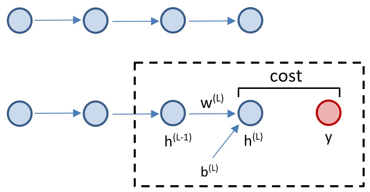
\(\frac{\partial J_1}{\partial w^{(L)}}\)

  • Changes in \(w^{(L)}\) influence \(z^{(L)}\) which in turn influences \(h^{(L)}\), which directly influences the cost \(J_1\). Formally:

$ = $

  • The above expression is known as chain rule of calculus and tells us the sensitivity of the cost function w.r.t. the weight \(w^{(L)}\)
  • It can be re-written as:

\(\frac{\partial J_1}{\partial w^{(L)}} = h^{(L-1)} \cdot g'(z^{(L)}) \cdot 2(h^{(L)} - y)\)

  • We can now average over all the \(n\) training examples (in the mini-batch), obtaining the total cost \(J\) for a batch of inputs:

\(\frac{\partial J}{\partial w^{(L)}} = \frac{1}{n} \sum_{i = 1}^{n} \frac{\partial J_i}{\partial w^{(L)}}\)

  • The above expression is just a component of the , which is composed of all partial derivatives of the cost function w.r.t. all weights and biases of the network:

\(\nabla_{\theta}J(\theta) = \Big[\frac{\partial J}{\partial w^{(1)}} \frac{\partial J}{\partial b^{(1)}} \frac{\partial J}{\partial w^{(2)}} \frac{\partial J}{\partial b^{(2)}} \frac{\partial J}{\partial w^{(3)}} \frac{\partial J}{\partial b^{(3)}} \Big]^T\)

  • Adjusting the other weights is slightly more complicated
  • First, we need an expression that determines the sensitivity of the cost \(J\) to the activation of the previous layer \(h^{(L-1)}\), that is:

\(\frac{\partial J_1}{\partial h^{(L-1)}}\)

\(= \frac{\partial z^{(L)}}{\partial h^{(L-1)}} \cdot \frac{\partial h^{(L)}}{\partial z^{(L)}} \cdot \frac{\partial J_1}{\partial h^{(L)}}\)

\(= w^{(L)} \cdot \frac{\partial h^{(L)}}{\partial z^{(L)}} \cdot \frac{\partial J_1}{\partial h^{(L)}}\)

  • Second, we apply again the chain rule:

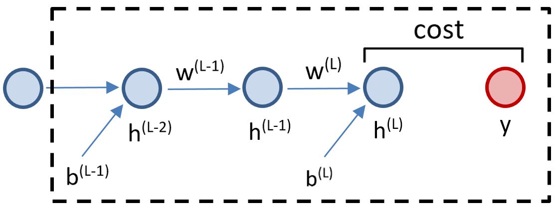
\(\frac{\partial J_1}{\partial w^{(L-1)}}\)

\(= \frac{\partial z^{(L-1)}}{\partial w^{(L-1)}} \cdot \frac{\partial h^{(L-1)}}{\partial z^{(L-1)}} \cdot \frac{\partial J_1}{\partial h^{(L-1)}}\)

\(= \frac{\partial z^{(L-1)}}{\partial w^{(L-1)}} \cdot \frac{\partial h^{(L-1)}}{\partial z^{(L-1)}} \cdot w^{(L)} \cdot \frac{\partial h^{(L)}}{\partial z^{(L)}} \cdot \frac{\partial J_1}{\partial h^{(L)}}\)

  • If we had more layers, we will keep repeating this idea by moving back into the network…

Gradient descent formulaic

  • The gradient gives us the direction of fastest increase of the function \(J\) at a point \(\theta\)
  • We can then move the parameters in the opposite direction from the gradient, thus decreasing the cost for a given batch
  • This approach is known as method of the steepest descent, or . Steepest descent proposes a new point:

\(\theta \leftarrow \theta - \epsilon \nabla_{\theta}J(\theta)\)

where \(\epsilon\) is the , a positive scalar determining the size of the step

  • If \(\epsilon\) is too small, the descent will take many iterations, and it could get stuck in a local minimum
  • If \(\epsilon\) is too large, the updates may end up taking us to completely random locations on the curve
  • Learning rate is one of the most difficult to set parameters because it affects model performance. There are several algorithms with adaptive learning rates
  • As the training set size grows, the time to take a single gradient step may become prohibitively long!
  • Deep neural networks are powered by stochastic gradient descent (SDG), essentially an extension of the gradient descent algorithm
  • The insight of SDG is that the gradient is an expectation, and this expectation can be approximately estimated using a small set of examples

  • On each step of the algorithm, we can sample a minibatch of examples \(\mathbb{B} = \{x^{(1)},...,x^{(m')}\}\) drawn uniformly from the training set (i.e. small number of examples, a few hundred max)
  • The estimate of the gradient is formed as:

\(g = \frac{1}{m'} \nabla_{\theta} \sum_{i = 1}^{m'} L(x^{(i)}, y^{(i)}, \theta)\)

  • …using the examples in the minibatch \(\mathbb{B}\)
  • Then we follow the estimated gradient downhill, that is:

\(\theta \leftarrow \theta - \epsilon g\)

  • We can now generalize to a network with more neurons
  • The cost \(J(\theta)\) can still be defined as a function of the parameters of the network (many more now)
  • The cost for a single training example is defined as:

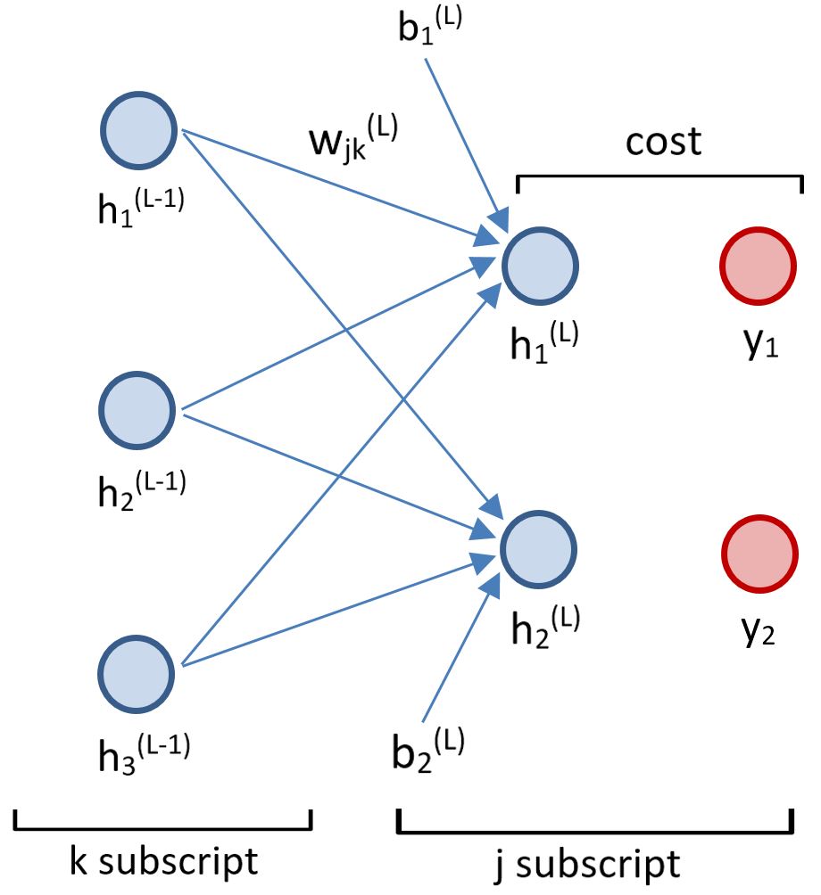
\(J_1 = \sum_{j = 1}^{n_L} (h_j^{(L)} - y_j)^2\)

  • Note that:

\(z_j^{(L)} = w_{j1}^{(L)} h_{1}^{(L-1)} + w_{j2}^{(L)} h_{2}^{(L-1)} + w_{j3}^{(L)} h_{3}^{(L-1)} + b_{j}^{(L)}\), and: \(h_{j}^{(L)} = g(z_j^{(L)})\)

  • Again, we can use the chain rule to figure out how sensitive the cost is to variations in a specific weight \(w_{jk}\):

\(\frac{\partial J_1}{\partial w_{jk}^{(L)}} = \frac{\partial z^{(L)}}{\partial w_{jk}^{(L)}} \cdot \frac{\partial h^{(L)}}{\partial z^{(L)}} \cdot \frac{\partial J_1}{\partial h^{(L)}}\)

  • We can repeat this process for all weights and biases feeding in a given layer; these partial derivatives determine the component of the gradient
  • What is changing here is the \(\frac{\partial J_1}{\partial h^{(L-1)}}\), since neurons influence the cost function through multiple paths. Formally:

\(\frac{\partial J_1}{\partial h_{k}^{(L-1)}} = \sum_{j = 1}^{n_L} \frac{\partial z_{j}^{(L)}}{\partial h_{k}^{(L-1)}} \cdot \frac{\partial h_{j}^{(L)}}{\partial z_{j}^{(L)}} \cdot \frac{\partial J_1}{\partial h_{j}^{(L)}}\)

  • Finally, the generic expression to update a weight in the layer \(\ell\) can be written as:

\(\frac{\partial J_1}{\partial w_{jk}^{(\ell)}}\)

\(= h_{k}^{(\ell-1)} \cdot g'(z_{j}^{(\ell)}) \cdot \frac{\partial J_1}{\partial h_{j}^{(\ell)}}\)

\(= h_{k}^{(\ell-1)} \cdot g'(z_{j}^{(\ell)}) \cdot \sum_{j = 1}^{n_{\ell+1}} w_{jk}^{(\ell+1)} \cdot g'(z_{j}^{(\ell+1)}) \cdot \frac{\partial J_1}{\partial h_{j}^{(\ell+1)}}\)

  • We can consider an additional hidden layer and adjust its weights
  • We obtain:

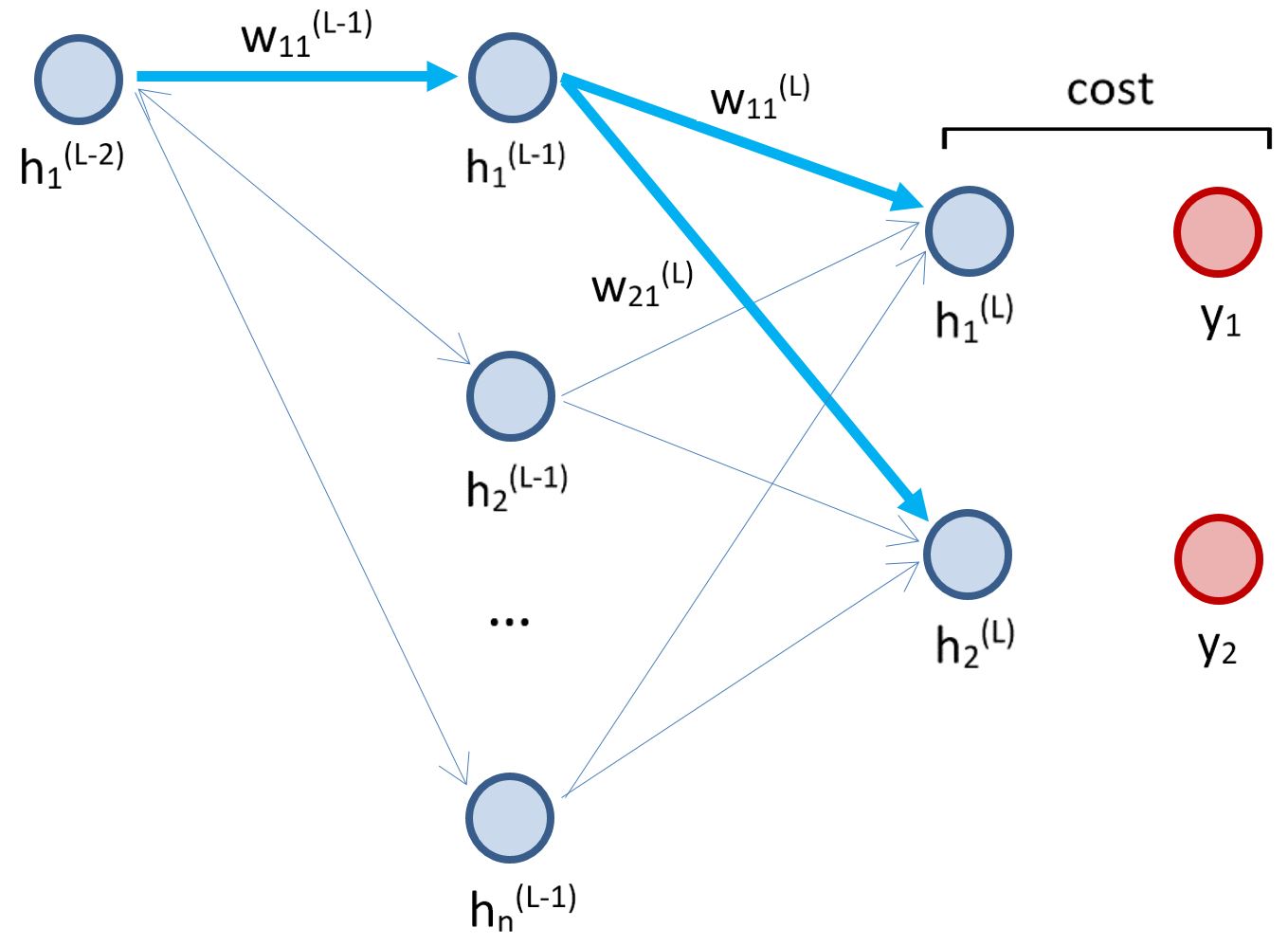
\(\frac{\partial J_1}{\partial w_{11}^{(L-1)}}\)

\(= h_{1}^{(L-2)} \cdot g'(z_{1}^{(L-1)}) \cdot \frac{\partial J_1}{\partial h_{1}^{(L-1)}}\)

\(= h_{1}^{(L-2)} \cdot g'(z_{1}^{(L-1)}) \cdot \sum_{j = 1}^{n_{L}} w_{j1}^{(L)} \cdot g'(z_{j}^{(L)}) \cdot \frac{\partial J_1}{\partial h_{j}^{(L)}}\)

  • We then average over all the examples in the minibatch