In this session, we will:

1. Reflect on sequential data and prediction problems.
2. Reviewing loops, and how they can be used to pass on information over time.
3. Introduce to Recurrent Neural Networks
4. Discuss their limits and the vanishing gradient problem
5. Introduce Long-short Term Menory (LSTM) Units

• A major characteristic of all neural networks you have seen so far, such as densely connected networks and convnets, is that they have no memory.
• Each input shown to them is processed independently, with no state kept in between inputs.
• This is fine for cross-sectional prediction problems such as identifying cats and dogs on pictures.
• However, many interesting real-life problems such as predicting stock prices, biofunctions, or the next word in a text are based on time-series or other types of sequential data.
• Information on past states of the outcome and/or other features often enhances performance, since these carry relevant information for future development.

• Using neural networks for such sequential problems, in order to process a sequence or a temporal series of data points, you have to show the entire sequence to the network at once: turn it into a single data point.
• Therefore, often we would like to operate over sequences of vectors: Sequences in the input, the output, or in the most general case both.

• Within human reasoning, we utulize information on past states naturally all the time.
• As you’re reading (or listening) the present sentence, you’re processing it word by word—or, keeping memories of what came before; this gives you a fluid representation of the meaning conveyed by this sentence.
• Biological intelligence processes information incrementally while maintaining an internal model of what it’s processing, built from past information and constantly updated as new information comes in. Our thoughts have persistence.
• Traditional neural networks can’t do this, and it seems like a major shortcoming. For example, imagine you want to classify what kind of event is happening at every point in a movie.
• Or a moving stock on the market, predicted just with a snapshot of its indicators at one point in time. It’s unclear how a traditional neural network could use its reasoning about previous events to inform later ones.

• Recurrent neural networks (RNN) address this issue in a very simplified way. They are networks with internal loops in them, allowing information to persist.
• it processes sequences by iterating through the elements and maintaining a state containing information relative to what it has seen so far.
• The state of the RNN is reset between processing two different, independent sequences, so you still consider one sequence a single data point: a single input to the network.
• What changes is that this data point is no longer processed in a single step; rather, the network internally loops over sequence elements.

state_t = 0 # the state as t

for (input_t in input_sequence) {
  output_t = f(input_t, state_t)
  state_t = output_t                   
}

• To make these notions of loop and state clear, let’s implement the forward pass of a toy RNN .
• This RNN takes as input a sequence of vectors, which you’ll encode as a 2D tensor of size (timesteps, input_features).
• It loops over timesteps, and at each timestep, it considers its current state at t and the input at t (of shape (input_features), and combines them to obtain the output at t.
• You’ll then set the state for the next step to be this previous output.
• For the first timestep, the previous output isn’t defined; hence, there is no current state. So, you’ll initialize the state as an all-zero vector called the initial state of the network.

state_t <- 0

for (input_t in input_sequence) {
  output_t <- activation(dot(W, input_t) + dot(U, state_t) + b)
  state_t <- output_t
}

• You can even flesh out the function f: the transformation of the input and state into an output will be parameterized by two matrices, W and U, and a bias vector b.
• It’s similar to the transformation operated by a densely connected layer in a feedforward network, right?

• Recurrent neural networks have the form of a chain of repeating modules of neural network.
• In standard RNNs, this repeating module will have a very simple structure, such as a single tanh() layer.
• It takes (differently) weighted input from the cells in the layer below, as well as of the state, which is just the “saved”/“remembered” layer below how it was one time-step earlier (at t-1).
• Then, with the tanh(), it squisches all the weights together to an output bounded between [-1,1].

• One of the appeals of RNNs is the idea that they might be able to connect previous information to the present task.

• Yet, going one step back is often not good enough, since meaning in some cases unfolds over a long sequence.

• We just stack several layer_simple_rnnon top of each other to capture the information contained in long sequences? Kind of, but there is a probhlem…

• In theory, RNNs are absolutely capable of handling such long-term dependencies.

• Sadly, in practice, RNNs don’t seem to be able to learn them. The problem was explored in depth by Hochreiter (1991, in German) and Bengio, et al. (1994)[^1], who found some pretty fundamental reasons why it might be difficult.

• First and foremost, the valishing gradient problem.

• Remember, the purpose of RNNs is to accurately classify sequential input.
• We rely on the backpropagation of error and gradient descent to do so.
• RNNs rely on an extension of backpropagation called backpropagation through time, or BPTT.
• Time, in this case, is simply expressed by a well-defined, ordered series of calculations linking one time step to the next, which is all backpropagation needs to work.
• Remember, neural networks, whether they are recurrent or not, are simply nested composite functions like y = f(g(h(x))).
• Adding a time element only extends the series of functions for which we calculate derivatives with the chain rule.

• Information flowing through neural nets passes through many stages of multiplication.
  
• Because the layers and time steps of deep neural networks relate to each other through multiplication, derivatives are susceptible to vanishing or exploding.
• This is an effect that is similar to what is observed with non-recurrent networks (feedforward networks) that are many layers deep: as you keep adding layers to a network, the network eventually becomes untrainable.
• Exploding gradients treat every weight as though it were the proverbial butterfly whose flapping wings cause a distant hurricane.
• Those weights’ gradients become saturated on the high end; i.e. they are presumed to be too powerful.
• But exploding gradients can be solved relatively easily, because they can be truncated or squashed. Vanishing gradients can become too small for computers to work with or for networks to learn – a harder problem to solve.

• Here you see the effects of applying a sigmoid function over and over again.
• The data is flattened until, for large stretches, it has no detectable slope.
• This is analogous to a gradient vanishing as it passes through many layers.

• Long Short Term Memory networks – usually just called LSTMs – are a special kind of RNN, capable of learning long-term dependencies.
• They were were introduced by Hochreiter & Schmidhuber (1997)[^2], and represent the cummulation of their work on the vanishing gradient problem. They work tremendously well on a large variety of problems, and are now widely used.
• After all, their idea was simple: They introduced a variant of layer_simple_rnn; it adds a way to carry information across many timesteps.
• Imagine a conveyor belt running parallel to the sequence you’re processing. Information from the sequence can jump onto the conveyor belt at any point, be transported to a later timestep, and jump off, intact, when you need it.
• This is essentially what LSTM does: it saves information for later, thus preventing older signals from gradually vanishing during processing.
• Remembering information for long periods of time is practically their default behavior, not something they struggle to learn!

• LSTMs also have this chain like structure, but the repeating module has a different structure.
• Instead of having a single neural network layer, there are four, interacting in a very special way.
• In adittion to the layer with the tanh() activation function that produces [-1,1] outputs, we see adittional sigmoid() layers that produce output between [0,1]

• Don’t worry about the details of what’s going on.
• We will do that one step by step. Lets get first comfortable with the notation:

In the above diagram, each line carries an entire vector, from the output of one node to the inputs of others.

• Pink circles represent pointwise operations, like vector addition
• Yellow boxes are learned neural network layers.
• Lines merging denote concatenation
• Line forking denote its content being copied and the copies going to different locations.

• The key to LSTMs is the cell state, the horizontal line running through the top of the diagram.
• The cell state is kind of like a conveyor belt. It runs straight down the entire chain, with only some minor linear interactions.
• It’s very easy for information to just flow along it unchanged.
• The LSTM does have the ability to remove or add information to the cell state, carefully regulated by structures called gates.

• Gates are a way to optionally let information through.
• They are composed out of a sigmoid neural net layer and a pointwise multiplication operation.
• The sigmoid layer outputs numbers between zero and one, describing how much of each component should be let through.
• A value of zero means “let nothing through,” while a value of one means “let everything through!”
• An LSTM has three of these gates, to protect and control the cell state.
  1. The Forget Gate
  2. The Input gate
  3. The Output Gate
• Conceptually, that is how an LSTM learns to remember as well as to forget. Lets inspect these layers more in detail.

• The first step in our LSTM is to decide what information we’re going to throw away from the cell state.
• This decision is made by a sigmoid layer called the **forget gate layer.*”** A 1 represents “completely keep this” while a 0 represents “completely get rid of this.”

Let’s go back to our example of a language model trying to predict the next word based on all the previous ones. In such a problem, the cell state might include the gender of the present subject, so that the correct pronouns can be used. When we see a new subject, we want to forget the gender of the old subject.

• The next step is to decide what new information we’re going to store in the cell state. This has two parts.
• First, a sigmoid layer called the input gate layer decides which values we’ll update.
• Next, a tanh layer creates a vector of new candidate values, Ct, that could be added to the state.
• In the next step, we’ll combine these two to create an update to the state.

In the example of our language model, we’d want to add the gender of the new subject to the cell state, to replace the old one we’re forgetting.

• It’s now time to update the old cell state, Ct−1, into the new cell state Ct.
• The previous steps already decided what to do, we just need to actually do it. We multiply the old state by ft, forgetting the things we decided to forget earlier.
• Then we add it∗Ct. This is the new candidate values, scaled by how much we decided to update each state value.

In the case of the language model, this is where we’d actually drop the information about the old subject’s gender and add the new information, as we decided in the previous steps.

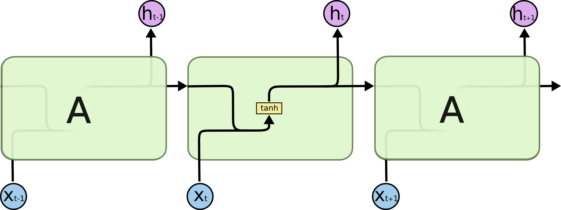
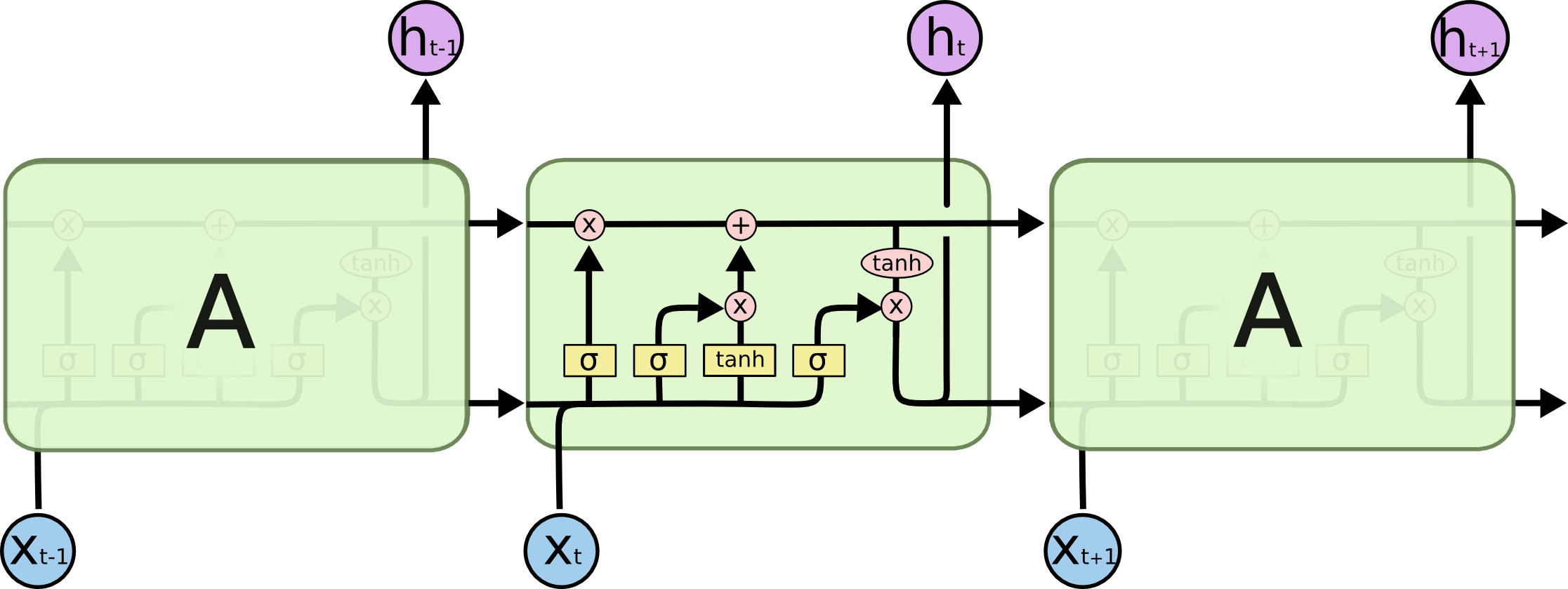
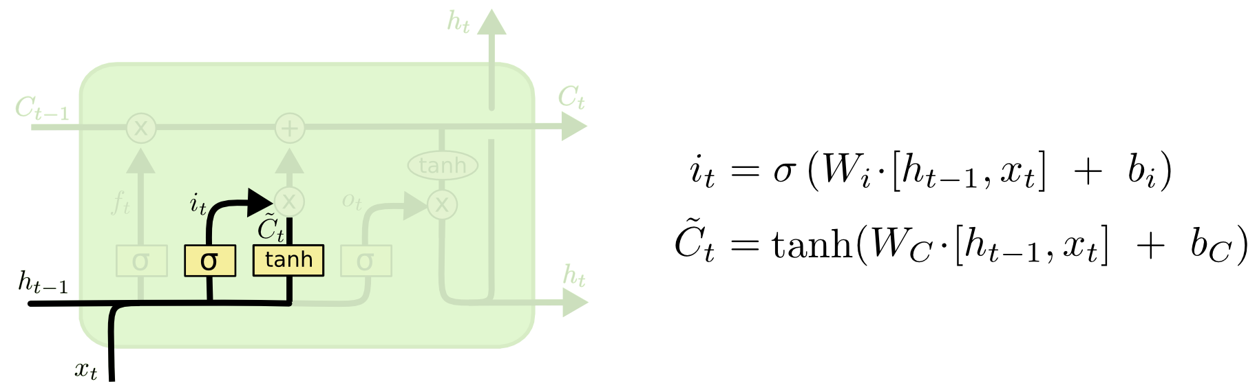
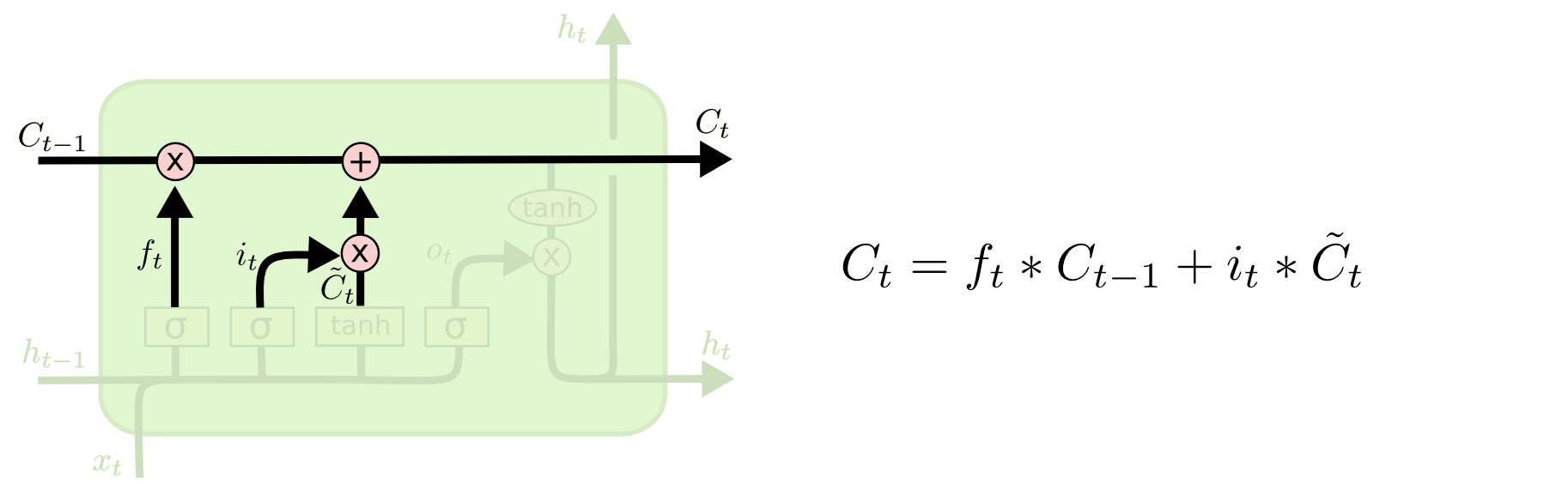
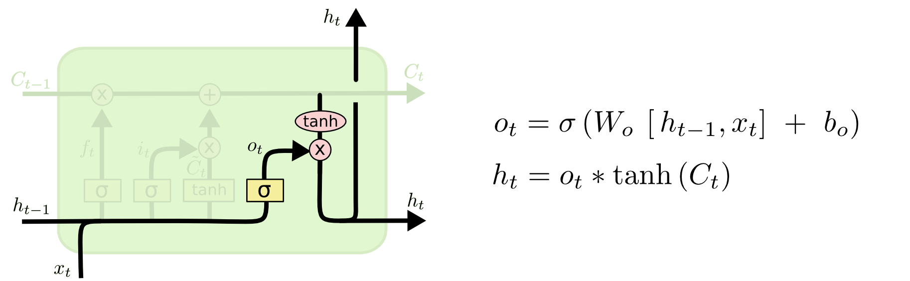
• Finally, we need to decide what we’re going to output. This output will be based on our cell state, but will be a filtered version.
• First, we run a sigmoid layer which decides what parts of the cell state we’re going to output.
• Then, we put the cell state through tanh (to push the values to be between [−1,1]) and multiply it by the output of the sigmoid gate, so that we only output the parts we decided to.

For the language model example, since it just saw a subject, it might want to output information relevant to a verb, in case that’s what is coming next. For example, it might output whether the subject is singular or plural, so that we know what form a verb should be conjugated into if that’s what follows next.

• And, thats pretty much it. Sounds complicated, and to some extent it is. However, the concept is pretty straightforward.
• In order to exploit the information of multiple recurrent layers, we have to find a way to train the weights while avoiding the vanishing gradient problem.
• Therefore we introduce gates, through which previous states can pass through quasi unaltered.
• However, not every information from previous sequences is useful for us. Indeed, too much information could be a curse rather than a blessing for our model.
• Therefore, we have to introduce further gates that decide which information from previous stages to remember, and which to forget.

We can envision the architectur of an LSTM as follows:

• Yoshua Bengio, Patrice Simard, and Paolo Frasconi, “Learning Long-Term Dependencies with Gradient Descent Is Difficult,” IEEE Transactions on Neural Networks 5, no. 2 (1994).
• Sepp Hochreiter and Jürgen Schmidhuber, “Long Short-Term Memory,” Neural Computation 9, no. 8 (1997).